That time I made a blog, added a few stars... and ended up ray-tracing black holes

At first the stars were meant to just twinkle behind the text. They learned to dodge the pointer, and it went to their heads: they formed a galaxy. The galaxy dispersed into comets and meteors of reality rejecting colors even though there’s no atmosphere to burn in. They needed somewhere to land, and the obvious choice is for them to crash into a black hole. There are two: the first doesn’t spin, and the second spins at 99.7% of the fastest rate possible, with every pixel’s light ray traced through its warped spacetime at whatever resolution your GPU agrees to.

You can go through the whole sequence on this page:

1. Hold the background (anywhere outside the text column) for about a second and a half: a galaxy forms where you pressed and stays. A quick click sends it back to the stars.
2. Scroll to tilt it. Keep scrolling and it gets stranger.
3. Press S to set off the comet/meteor shower.
4. Press S again to feed it to a black hole. During the close-up, B switches between the two black holes.
5. Press S a third time to pull back out to the galaxy.

While the galaxy is on screen:

• Drag, or use the arrow keys, to spin it.
• X, Y and Z spell out that Pauli gate in its stars. The same key again dismisses it.

Most sections have a live demo that shows how the colored symbols in the text relate to what is being drawn, labeling each with its live value. The demo’s Equations button turns the colors and labels off. A vector is written with an arrow, as in a position $\vec{r} = (x, y)$vector r equals x, y, and a unit vector (of length 1) as $\hat{r}$r hat. Plain letters are single numbers, except the Pauli matrices and the indexed quantities of relativity, which their sections introduce. A field is a quantity with a value at every point, such as a pattern of noise or the curvature of spacetime. While I won’t derive everything from scratch, the included references point at where complete derivations for some key results can be found.

The idle sky

Before anything is pressed, the background is a 2D canvas of stars that twinkle, scatter from the pointer and now and then gather into a diagram. Each star’s opacity swings around a base value on a sine of its own rate, so no two stars blink together.

Each star carries three vectors in screen pixels: its home $\vec{h}$vector h, its position $\vec{r}$vector r and its velocity $\eq{v}{\vec{v}}$vector v, in pixels per frame. Every frame the code updates the velocity and then the position, with $\leftarrow$the left arrow meaning “replace with” and $\Delta t$delta t, one frame, the time step:

The velocity update adds the pointer’s force $\eq{F}{\vec{F}}$vector F over one step to the velocity and multiplies the sum by $\eq{mu}{\mu} < 1$mu less than 1, a friction. The position update moves the star by its velocity over one step, and a spring pulls it a fraction $\eq{lambda}{\lambda}$lambda of the remaining way to its anchor $\eq{g}{\vec{g}}$vector g, which is normally its home.

The force pushes straight away from the pointer and falls off linearly to zero at a radius $\eq{R}{R}$R, beyond which it vanishes:

where $d$d is the star’s distance from the pointer, $\hat{r}$r hat the unit vector pointing away from it and $F_0$F zero the force at the pointer itself.

Friction caps the speed: under a steady push the velocity grows until friction takes away as much each frame as the force adds. A pointer slower than that cap keeps the stars ahead of it in reach and herds them along, and a quick one passes through them and barely moves them. Once the pointer has gone, friction soon stops the star and the spring takes it home. Each frame the spring closes the same fraction of the remaining distance, so the star moves fastest far from home and slows as it arrives.

The diagrams are six quantum circuits that form in a side margin, the first as soon as the page loads. Each is a set of points, and the stars nearest its center swap their anchor $\eq{g}{\vec{g}}$vector g from home to one point each. The same spring, with a larger $\eq{lambda}{\lambda}$lambda, pulls them into the drawing. Taking the nearest stars keeps every flight short, and the diagram condenses out of the stars around it. It holds until the pointer comes close or a scroll carries it out of view. Then each star’s anchor returns to its home, the stars fly back, and the next diagram waits until they have all arrived.

The galaxy

The idle sky updates each star on the CPU in screen pixels, which suits a sparse field in two dimensions. The galaxy has thousands of stars that must follow curved arms, turn in three dimensions and react to scrolling, so it divides the work. A star stores no position of its own, only the curve it rides, called its stroke, and its progress along that stroke. The CPU builds the strokes once. Each frame the GPU draws the stars with two small programs, called shaders: a vertex shader finds each star’s place on its stroke and so on the screen, and a fragment shader colors each pixel the star covers. Values that are the same for every star in a draw, such as the time, are called uniforms.

Strokes as paths

Each arm is a logarithmic spiral: its radius $r$r grows exponentially with the angle $\theta$theta, from $r_0$r zero at $\theta = 0$theta equals 0, at a rate that drops from $b_1$b one to $b_2$b two at a break radius $\eq{r1}{r_1}$r one, which the arm reaches at angle $\theta_1$theta one:

The steep inner segment packs a compact core, and the shallow outer one winds the arm more tightly, in a long curve around it. Three arms start a third of a turn apart, a fourth stroke runs a second outer spiral alongside one of them, and three short spirals fill the core.

A star needs a position at every progress value $\eq{s}{s} \in [0, 1]$s between 0 and 1 along its stroke. The stroke’s points are joined by a Catmull-Rom curve, a smooth curve through all of them. It traces $\vec{C}(\eq{u}{u})$vector C of u as a parameter $\eq{u}{u}$u runs from 0 to 1, with an equal share of $\eq{u}{u}$u for each segment between two points. That parameter does not measure distance: a star moving at a constant rate in $\eq{u}{u}$u would speed up and slow down along the stroke. The path code therefore measures arc length,

numerically from a dense polyline, and resamples the curve at equal steps of $\eq{s}{s}$s. A constant rate in $\eq{s}{s}$s is then a constant speed.

Each star draws a seed $q$q uniformly from $[0, 1]$0 to 1, which is then warped by an amount $\eq{f}{f}$f between 0 and 1:

Where $d\eq{s}{s}/dq$d s by d q is small, many seeds land on a short stretch of stroke. The derivative is smallest at $q = 1/2$q equals one half, which crowds stars into the middle of each stroke and thins them toward both ends.

Every stroke flows inward by advancing its seeds at its own rate, $\dot q = c$q dot equals c, and inner and outer strokes lap each other. Progress along the stroke then moves at $\dot{\eq{s}{s}} = c\,(1 + \eq{f}{f} \cos 2\pi q)$s dot equals c times 1 plus f cosine 2 pi q, slowest in the middle, so stars slow down where they crowd and the crowd stays in place. Far from the center, stars also slow down by a factor

where $r$r is the star’s distance from the center and $\mathrm{smoothstep}(a, b, x) = y^2 (3 - 2y)$the smoothstep of x between a and b equals y squared times 3 minus 2 y, with $y = (x - a)/(b - a)$y equals x minus a, over b minus a clamped to $[0, 1]$0 to 1, rises from 0 at $a$a to 1 at $b$b with zero slope at both ends. Between the radii $r_a$r a and $r_b$r b the speed falls to half. The outer stars trail the inner ones, and the galaxy never turns as a rigid body.

The resampled points of every stroke go into a small texture, an image the shaders can read. The vertex shader computes a star’s position from that texture, the star’s seed and a few uniforms such as the time, the scroll and the intro progress, so steady motion sends the GPU at most one number per star each frame.

Stars on the GPU

Each star twinkles on a sine of its own frequency, as in the 2D field. The galaxy renders into a high-dynamic-range image, whose brightness can exceed what the screen shows. A bloom pass blurs the brightest stars into a glow at several scales, and a filmic tone curve compresses the result into the screen’s range.

When the galaxy appears, every star starts at a random point inside a circle of radius $r_\text{max}$r max. Drawing the radius as $r = r_\text{max}\sqrt{w}$r equals r max times the square root of w with $w$w uniform on $[0, 1]$0 to 1 spreads the stars evenly over its area: the fraction inside radius $r$r is then $(r/r_\text{max})^2$r over r max, squared, exactly the fraction of the area. Each star then slides to its place on its stroke in a time window of its own within the first few seconds of the intro clock $\eq{tintro}{t_\text{intro}}$t intro, swinging around the center by an angle that rises and falls back to zero on the way, so the field spirals into place instead of dropping straight onto the arms.

Scrolling drives the rest. As the scroll progress $\eq{chi}{\chi}$chi goes from 0 to 1, the galaxy tilts and then eases back flat. Later in the scroll the stars leave their strokes: each moves a share $\eq{sigma}{\sigma}$sigma of the way from its place on its stroke to a new position,

and $\eq{sigma}{\sigma}$sigma rises smoothly from 0 to nearly 1 by the end of the scroll while the galaxy dims. One star in four ends up scattered around the galaxy. The other three form a DNA double helix that winds along an S through the galaxy’s center and turns slowly: two backbones a little under half a turn apart, as in DNA, with base pairs between them.

Some effects run on the CPU and need to know where the stars are: the pointer’s push, the lens flares on the brightest stars, and the meteor shower, which launches from the stars’ current positions. A CPU mirror of the vertex shader therefore recomputes every star’s position with the same formulas, and the two copies have to agree.

For a while they did not, and the push hit the wrong stars: a sweep of the pointer kicked stars it never passed over and missed the ones it did. The shader took each star’s scatter seeds from a popular GPU hash, the fractional part of $43758.5453 \sin z$43758.5453 times the sine of z, with $z$z built from two of the star’s attributes. Its author is unknown: it has been copied from shader to shader for at least fifteen years, and Google’s Skia graphics library calls it a function “floating around on the internet”. The large factor amplifies the last digits of the sine. Those are exactly the digits where the GPU’s 32-bit sine and the CPU’s 64-bit one disagree, so the shader and the mirror drew different seeds and put the stars in different places. The seeds are now drawn once on the CPU and passed to the shader with each star.

When the pointer moves by $\Delta \vec{p}$delta p, every star near its path gets a kick to its velocity along that motion,

where $d$d is the star’s distance from the pointer’s path, $\eq{R}{R}$R the reach of the push, $J_0$J zero its strength and $m$m a mass that grows with the star’s size. The kick adds to the star’s velocity $\eq{v}{\vec{v}}$vector v, and its offset $\eq{x}{\vec{x}}$vector x from its place in the galaxy evolves as

where dots indicate time derivatives. The velocity dies away at the damping rate $\gamma$gamma, and the offset follows it back to zero over a time $t_0$t zero. Mass sets how a star takes a push: a light one gets a large kick and loses it quickly, a heavy one gets a small kick and glides on longer. Both equations are linear and have an exact solution, and each frame moves every star along it by the time that actually passed. The push therefore plays out at the same pace at any smooth frame rate. The 2D field instead takes one fixed step per frame and runs twice as fast on a 120 Hz screen as on a 60 Hz one.

The Pauli gates

X, Y and Z gather the galaxy’s stars into that Pauli gate’s matrix, with $i$i the imaginary unit:

Each matrix is written in a single-line stroke font whose strokes are resampled by arc length like the galaxy’s strokes. The stars are shared out over the strokes by length, so every glyph comes out evenly dense, and each star is given a point on its stroke, with a small random offset across the stroke that gives each line some width. A spring pulls the star from its place in the galaxy toward its point, and the gap shrinks as $e^{-kt}$e to the minus k t. The spring’s strength $k$k rises from zero as the gate forms while the points grow from the screen’s center to full size, so the gate grows out of the galaxy.

Once the gate has formed, the points walk along the strokes and the spring keeps each star on its point. A point with phase $\eq{phi}{\varphi}$phi, a fraction of a lap, on a stroke of length $\eq{L}{L}$L, moving at speed $c$c, sits at time $t$t at arc fraction

where $\operatorname{frac}(x) = x - \lfloor x \rfloor$the fractional part of x equals x minus the floor of x is the fractional part. On a closed stroke, $\eq{phi}{\varphi} + ct/\eq{L}{L}$phi plus c t over L counts laps, and its fractional part is how far along the current lap the star is. Because the stroke’s end joins its start, the star circles it without a jump. An open stroke’s ends are apart, so the star walks out and back instead: with $\eq{u}{u} = \operatorname{frac}(\eq{phi}{\varphi} + ct/(2\eq{L}{L}))$u equals the fractional part of phi plus c t over 2 L the share of the current lap done, $1 - \lvert 1 - 2\eq{u}{u} \rvert$1 minus the absolute value of 1 minus 2 u runs from 0 to 1 and back to 0 as $\eq{u}{u}$u runs through a lap. That round trip covers the stroke twice, hence the $2\eq{L}{L}$2 L.

The pointer can still knock stars off their points, and the spring draws them back. Releasing the gate lets the stars return to the galaxy.

Meteors, comets and their trails

So far every star has stayed in the galaxy or on a gate. Pressing S breaks a fraction of them free as a shower of meteors and comets. Each object starts where its star was at that moment, read from the CPU mirror, and flies in a straight line. All the objects travel in roughly the same direction. The scene uses an orthographic camera, which has no perspective of its own, so the code applies a per-object depth $\eq{D}{D}$D by hand to the sprite size $\eq{S}{S}$S and the screen speed $\eq{V}{V}$V:

where $S_0$S zero and $V_0$V zero are the size and speed at depth 1. A pinhole camera produces the same pair: an object twice as far away looks half as large and crosses the screen at half the speed. An object that leaves one edge respawns at the other at a new height.

Most of the shower is white shooting stars. A few objects, picked at random, take the galaxy’s rare star colors (blue, purple and a single orange) and burn as meteors with smoky trails. Three comets fly with them. The GPU draws each object as a sprite, a small square patch of the screen, and the fragment shader sets the brightness of every pixel in it. It lights a thin streak along the direction of motion and leaves the rest of the square dark, so the square’s edges never show. To place the streak, the shader measures each pixel’s position $\vec{p}$vector p from the sprite’s center, in sprite widths, along the direction of motion $\eq{d}{\hat{d}}$d hat and across it, along $\eq{d}{\hat{d}_\perp}$d perpendicular:

The coordinate $\eq{a}{a}$a runs from $-\tfrac12$minus one half at the tail to $\tfrac12$one half at the front. A shooting star’s brightness rises from zero at the tail as a power of $\eq{a}{a} + \tfrac12$a plus one half to a Gaussian head near the front, and a Gaussian in $\eq{c}{c}$c narrows it to a thin line. A taper takes it to zero before the edge of the square, which keeps the sprite’s outline from showing.

A halo around the head splits into color channels. The shader evaluates one Gaussian $g$g three times, shifted across the path by a small $\epsilon$epsilon, different for each object, and sends one copy to each color channel, scaled by that channel of the object’s color $(k_R, k_G, k_B)$k R, k G, k B:

Near the center the three copies overlap and return the object’s own color. At the rim one side keeps mostly red and the other mostly blue, the fringe that chromatic aberration leaves around a bright point. The scene has no lens, and the shader adds its flaw anyway. The whole shower blends additively: where two objects cross, their light adds, and the draw order has no effect.

Trails that stay in the sky

Meteors and comets replace the streak with a head, a coma (the soft glow around it) and a trail, drawn by one shared function in which they differ only by a stretch factor. A comet’s sprite is larger by that factor, and the shader shrinks the head and the trail’s width back by the same factor, so only the trail lengthens. A meteor’s short, turbulent trail reads as flame, a comet’s long, even one as a tail. Astronomers separate them by what they are: a comet is an icy body in orbit, a meteor a grain burning up in an atmosphere.

The trail is a function of the distance $b$b behind the head along $-\eq{d}{\hat{d}}$minus d hat, the offset $c$c across the path, and the head’s travel $\eq{T}{T}$T, how far it has flown so far. With $\ell$ell the trail’s length, the age $\eq{alpha}{\alpha} = \min(b/\ell, 1)$alpha equals the smaller of b over ell and 1 runs from 0 at the head to 1 at the end, since smoke farther back left the head earlier. The trail’s width and center line are powers of the age:

Here $w_0$w zero is the width at the head, $W$W the width the trail gains by its end and $C$C how far its center line has bent by then. At $\gamma = \tfrac12$gamma equals one half the smoke spreads like a diffusing puff, whose width grows as the square root of time, and at $\gamma = 1$gamma equals 1 it spreads linearly, as a turbulent jet does. Each trail picks $\gamma$gamma at random from a range that spans both. An exponent $\eta$eta above 1 keeps the trail straight as it leaves the head and bends it further back, toward a random side.

Inside that outline, the smoke’s texture is noise sampled in coordinates that follow the trail’s shape, with scales $s_1$s one along the path and $s_2$s two across it and a drift factor $\eq{kappa}{\kappa}$kappa:

Dividing by $\eq{w}{w}$w stretches the noise across the path as the trail widens, and the smoke’s features grow with it. The first coordinate sets how the smoke moves across the sky. Measured in sky positions along the path, the head started at $X_0$X zero and now sits at $X_h = X_0 + \eq{T}{T}$X h equals X zero plus T, and a point $b$b behind it sits at $X = X_h - b$X equals X h minus b. Substituting,

For $\eq{kappa}{\kappa} = 1$kappa equals 1 the noise coordinate depends only on the sky position $X$X. The smoke stays where the head released it and the head draws away from it, which is how a real trail behaves in still air. With $\eq{T}{T}$T frozen, the pattern would instead ride along with the head as a painted streak. Each trail picks a random $\eq{kappa}{\kappa}$kappa close to 1, so its smoke drifts slowly after the head ($\eq{kappa}{\kappa} < 1$kappa less than 1) or streams back ($\eq{kappa}{\kappa} > 1$kappa greater than 1).

The substitution requires $b$b and $\eq{T}{T}$T in the same unit. The shader measures $b$b in the sprite’s own coordinates, so the CPU accumulates the object’s screen speed $V$V divided by its sprite size over time $t$t:

The speed and the sprite size share the factor $1/D$1 over D, so the integrand does not depend on depth, and near and far objects shed smoke at the same rate relative to their size.

Smoke layers

One sample of gradient noise $n$n, a smooth random field over the plane, gives smooth blobs. The shader folds them by domain warping [1]: two samples form a displacement $\eq{e}{\vec{e}}$vector e, and the final sample $\eq{nu}{\nu}$nu is read at the displaced point,

where the offset $\vec{\xi}_0$xi zero decorrelates the two samples and $\eq{lambda}{\lambda}$lambda sets how far the warp displaces the final one. Where $\eq{e}{\vec{e}}$vector e changes quickly, neighboring pixels read distant parts of the noise, and the blobs fold into curls and tendrils. The warp also bends the trail: its first component moves the center line by $\delta = e_x\, \eq{w}{w}\, h(\eq{alpha}{\alpha})$delta equals e x times w times h of alpha, where $h$h rises from zero near the head, so the smoke meanders more the older it is.

Three layers are drawn from this field, named after a real comet’s tails: a broad, curving tail of dust and a thin, straight tail of ions with fine filaments along it. The dust is a Gaussian across the trail, centered on the curled line $\eq{c0}{c_0} + \delta$c zero plus delta, and $\eq{nu}{\nu}$nu breaks it into lumps. The ion strand and the filament are much thinner Gaussian threads that follow the dust’s curl only partly and stay unbroken where the dust breaks up. The filament leans away faster, so it peels off the ion strand as the trail ages.

The three layers are summed with random weights per trail and multiplied by a fade $(1 - \eq{alpha}{\alpha})^{\psi}$1 minus alpha, to the psi, which takes the trail to zero at its end. The dust’s brightness alone is also multiplied by a pattern of bright bands spaced along the trail, as real dust tails show:

with depth $\epsilon_P$epsilon P, spacing $2\pi / f_P$2 pi over f P and phase $\varphi$phi. By the substitution above, the crests move over the sky at $1 - \kappa_P$1 minus kappa P of the head’s speed. With $\kappa_P$kappa P below 1 they drift forward more slowly than the head, and relative to the head they run back down the trail.

From the shower to a black hole

A second S ends the shower by pulling it into a black hole. Every object gets a target orbit radius, spaced with the golden ratio so the orbits spread evenly across the disk instead of bunching up, and an angular speed that follows Kepler’s third law from a speed $\omega_0$omega zero at radius $r_0$r zero,

clipped near the center, where Kepler would ask for an infinite speed. Each object’s radius relaxes toward the target.

The objects gather into the accretion disk, the gas orbiting the hole. Gravity bends light, so a camera near the hole sees that disk distorted, its far side lifted over the hole. Each object is drawn where the camera sees its point of the disk.

As an object settles onto its orbit, it hands its mass to a coarse polar grid. Its sprite fades out, and its light passes to a finer map of the disk’s glow, so the object joins the disk as a bright knot that turns with the gas and blends in over a few seconds. While it spirals in, it also paints a fading streak along its path into the same map, so fast objects trail glowing filaments through the disk. The grid holds the mass and decides where the disk is, and the map holds the light that makes the knots and streaks glow.

The grid then turns with the disk: the same law $\eq{omega}{\omega}(r)$omega of r, with the smaller $\omega_0$omega zero at which the Schwarzschild model’s gas flows. In a frame of duration $\Delta t$delta t, each ring shifts by $\eq{omega}{\omega}(r)\,\Delta t$omega of r times delta t in angle, a fraction $\eq{delta}{\delta}$delta of a sector, and linear interpolation gives each sector $j$j of the ring, holding mass $\eq{m}{m_j}$m j, its new mass $\eq{m}{m_j}'$m j prime:

Each cell’s mass splits between itself and its neighbor, so every ring keeps its total, and a ring that caught nothing stays empty. Both black-hole models draw their disk from this grid, which puts the disk where the matter arrived.

The camera zooms in on the hole and holds the close-up until the next S. The hole and its disk are drawn in a layer of their own, and the pullback takes that layer’s magnification $\eq{z}{z}$z from its close-up value $z_0$z zero down by a total factor $Z$Z,

where $\eq{q}{q}$q runs from 0 to 1 over the pullback and the smoothstep $\eq{rho}{\rho}$rho eases it at both ends. Near the end of the pullback the hole fades out, and the galaxy is left on its own.

During the close-up the galaxy keeps moving behind the hole as its sky. Its stars render into an offscreen texture instead of the screen. The black-hole shader traces each pixel’s ray, and where the ray escapes, it reads that texture where the bent ray points. The sky is magnified along with the view, and so is its motion, which would blur its arms. Its clock runs slower by that magnification instead, which keeps the stars at their usual pace on screen, and speeds back up as the camera pulls out. It’s the only instance of time dilation on the site with an editorial cause.

Two black holes

Successive captures take the two models in turn, and B switches between them during the close-up. They share everything above: the captured-matter grid, the lensed galaxy sky and the pullback. The Schwarzschild model reads its light paths around a hole without spin from a table of the exact orbit equation, computed once. The Kerr–Newman model integrates the geodesic equations for each ray around a hole with spin and charge, and per traced pixel it costs about sixty times as much.

Tracing and marching

In computer graphics, ray tracing sends a straight line from the camera through each pixel and solves for the first surface it meets. A sphere or a triangle gives an equation in the distance along the line, and its smallest positive root is the hit. Around a black hole neither part works. Light bends, so no formula gives where a ray is after a given distance, and in the Kerr–Newman model the disk is gas, with no surface to hit.

The Kerr–Newman model therefore follows each ray from the camera in steps, each advancing its position and direction a short distance by its equation of motion. Graphics calls stepping along a ray ray marching and uses it for fog, smoke and other volumes, where a ray gathers light from every point it passes. Relativists use ray tracing for the whole procedure of following light back from the camera through curved spacetime, whatever method computes the path. GYOTO, a code that renders black holes, calls itself “a general relativistic ray-tracing code” [2].

Two choices set what a model computes: how it finds the path, and whether its matter is a surface to intersect or a volume to sample, at a cost that grows with the length of gas a ray crosses. The Schwarzschild model’s disk is a thin slab, a surface. Its rays are looked up instead of stepped, and each crossing of the slab is solved for directly: classic ray tracing on a curved path. The Kerr–Newman model’s disk is a volume, sampled at intervals along each straight segment between its steps: tracing for the path, marching for the matter.

Whichever way a model finds its gas, both accumulate light along a ray the same way. Walking from the camera outward, the ray gathers a color $C$C and an opacity $A$A, color channel by color channel, and each sample of gas with color $c_i$c i and opacity $a_i$a i adds only what the gas in front of it has not already covered:

Schwarzschild: a table of light paths

Around a non-rotating black hole with Schwarzschild radius $R_s$R s, light follows paths whose inverse radius $u = 1/r$u equals 1 over r, as a function of the angle $\varphi$phi around the hole, obeys

A ray stays in the plane through the hole and its starting direction, and the camera’s distance from the hole is fixed, so one number sets the ray’s path in that plane: its impact parameter $\eq{b}{b}$b, the distance at which its straight line would pass the hole.

Far from the hole the orbit equation’s right side is small. Without it, $u = \sin\varphi / \eq{b}{b}$u equals sine phi over b is a straight line. To first order the right side adds $\tfrac{R_s}{2\eq{b}{b}^2}(1 + \cos^2\varphi)$R s over 2 b squared, times 1 plus cosine squared phi, which turns both ends of the line, where $u = 0$u equals 0, toward the hole by $R_s/\eq{b}{b}$R s over b, a total deflection

Einstein’s light bending for a mass $M$M, since $R_s = 2GM/c^2$R s equals 2 G M over c squared. At $r = \frac{3}{2} R_s$r equals three halves R s, the photon sphere, light can circle the hole on an unstable orbit. A ray with the critical impact parameter $\eq{b}{b} = \frac{3\sqrt{3}}{2} R_s$b equals 3 root 3 over 2, times R s winds ever closer to that orbit, rays with smaller $\eq{b}{b}$b spiral into the hole, and together they form its shadow, whose edge the critical rays mark.

When the page loads, the code integrates the orbit equation outward from the camera for a few hundred impact parameters, crowded toward the critical value, where a small change in $\eq{b}{b}$b changes the path most. It stores $u$u and its derivative along each path over two turns, with the angle at which the path escapes or falls in. The shader computes each pixel’s $\eq{b}{b}$b and the plane its ray turns in, and reads the path from the table, interpolating between neighboring entries. The ray’s plane meets the disk along a line through the hole, so the ray can cross the disk only where it passes that line, once every half turn. The table gives its radius at each crossing.

My first version stepped each ray through an ordinary central force whose paths are the same, as Riccardo Antonelli’s Starless ray tracer does [3]. I used leapfrog, a simple step-by-step integrator, and a ray took dozens of steps. When I replaced the stepping with the table, it drew the hole about four times faster, since a crossing costs four texture reads.

The table also turned out more accurate. I checked both against the same orbit equation integrated in tiny steps for each pixel’s own ray. The table places the disk’s images and the lensed sky within a fraction of a pixel, and the shadow’s edge is exact, since whether a ray falls in follows from $\eq{b}{b}$b alone. The leapfrog was off by as much as 21 pixels in the sky near the critical value, where lensing squeezes the whole sky into a sliver, and it missed the thin ring.

The lensed sky follows from where each ray ends up. A ray aimed at an angle $\eq{theta}{\theta}$theta from the hole, with the camera at a distance $D$D, passes at $\eq{b}{b} \approx D\eq{theta}{\theta}$b roughly D theta and is bent back by $\eq{alpha}{\alpha}$alpha, so it sees the sky at

This is the lens equation. A star directly behind the hole, $\eq{beta}{\beta} = 0$beta equals 0, appears on the Einstein ring $\eq{theta}{\theta} = \eq{thetaE}{\theta_E}$, smeared all the way around it. The galaxy’s bright core sits exactly behind the hole and would smear into a thin bright ring, so near $\eq{beta}{\beta} = 0$beta equals 0 the shader reads a blurred copy of the sky.

Because the disk is far thinner than it is wide, the light through it at each crossing has a closed form: a slab of column density $\Sigma$Sigma, crossed at an angle whose cosine to its normal is $\eq{mu}{\mu}$mu, has optical depth and opacity

where $\kappa$kappa is the gas’s absorption per unit column density, so each crossing is one sample $a_i$a i of the sum above. The column density comes from the matter grid at the crossing, shaped by a noise texture.

The gas moves on circular Kepler orbits, and its light arrives shifted in frequency. With $\eq{g}{g}$g the ratio of observed to emitted frequency, above 1 when the light arrives bluer, a photon whose angular momentum about the disk’s axis is $\eq{xi}{\xi}$xi per unit energy has

Here $M$M is the mass in units where $G = c = 1$G and c equal to 1 and $\eq{Omega}{\Omega}$Omega the gas’s angular speed. The numerator is the time dilation of an orbit at radius $r$r, and the denominator is the Doppler factor of the gas’s motion along the photon, as in Luminet’s 1979 image of a thin disk around such a hole [4].

The disk fades in across the innermost stable circular orbit, $\eq{rin}{r_\text{in}} = 3 R_s$r in equals 3 R s: inside it no circular orbit is stable, and gas plunges into the hole instead of orbiting. Its temperature follows the thin-disk profile [5]

Its color comes from a warm palette indexed by the observed temperature $\eq{g}{g} \eq{T}{T}$g T, relative to the disk’s peak. Its brightness at frequency $\nu$nu, the specific intensity $I_\nu$I nu, scales as $\eq{g}{g}^3$g cubed, because $I_\nu / \nu^3$I nu over nu cubed is conserved along a ray.

The gas’s noise is a sum of octaves, layers of detail at finer and finer scales. Where one pixel covers a long stretch of disk, seen edge-on, squeezed against the shadow or sheared near the inner edge, the finest octaves would flicker, so the shader fades out those finer than the jump in noise coordinates from one pixel to the next, as a mipmap (a texture’s stack of ever blurrier copies) does.

Rays near the critical impact parameter circle the hole before leaving, and each extra half turn shows another, thinner image of the disk. Each time a ray’s impact parameter gets $e$e times closer to the critical value, the ray winds one more radian around the hole. The disk’s next image lies another half turn on, $\pi$pi radians, so it takes rays $e^\pi \approx 23$e to the pi, about 23 times closer, and each image is about 23 times thinner than the one outside it. Above the shadow in the close-up, one image is a few pixels wide, and the next, a ring thinner than a pixel, lies just outside the shadow. One ray per pixel would catch such a ring only here and there, so a pixel whose ray passes near the critical impact parameter averages a grid of extra rays across itself, which also softens the shadow’s edge.

A disk that does not wind up

The noise texture that gives the gas its structure has to orbit with the matter, fast near the hole and slowly far out. The obvious way is to read the texture at the angle $\varphi = \gamma - \eq{omega}{\omega}(r)\,\eq{t}{t}$phi equals gamma minus omega of r times t, where $\gamma$gamma is the point’s angle around the hole, $\eq{omega}{\omega}(r)$omega of r the texture’s angular speed at radius $r$r, the matter grid’s rate, and $\eq{t}{t}$t the time. Two nearby radii then separate in angle at the rate

which grows without bound. My first attempt at the disk did exactly this: within seconds of a capture, neighboring radii read unrelated noise, and the disk showed hundreds of concentric bands. Real gas winds too. A noise texture wound this far, though, looks like a vinyl record.

The fix bounds the shear. Two texture layers, $k = 0$k equals 0 and $1$1, each rotate at the local rate for a period $\eq{P}{P}$P and then restart on fresh noise, half a period apart, with $\eq{tk}{t_k}$t k the time since layer $k$k last restarted:

The angle a layer turns is then at most $\eq{omega}{\omega}(r) \eq{P}{P}$omega of r times P, so its shear stays below $\tfrac32 \eq{omega}{\omega}(r) \eq{P}{P} / r$three halves omega of r P over r. A fixed term $\psi(r) \propto r^{-1/2}$psi of r proportional to one over the square root of r gives the texture a trailing spiral that doesn’t grow. Locally the gas still moves at $\eq{omega}{\omega}(r)$omega of r.

The layers cross-fade with triangular weights $\eq{w}{w}$w and $1 - \eq{w}{w}$1 minus w, and each layer restarts at the moment its weight is zero. Mixing two independent noises this way lowers the contrast: the mix’s variance is $\eq{w}{w}^2 + (1 - \eq{w}{w})^2$w squared plus 1 minus w, squared times one noise’s, half at the crossover. Dividing the mix by $\sqrt{\eq{w}{w}^2 + (1 - \eq{w}{w})^2}$the square root of w squared plus 1 minus w, squared restores it, so the texture looks the same throughout a capture, with no pulse at the restarts.

Kerr–Newman

The second model traces light through the Kerr–Newman metric of a hole with mass $M$M, spin $\eq{a}{a}$a and electric charge $\eq{Q}{Q}$Q. The site runs it at $\eq{a}{a} = 0.997M$a equals 0.997 M and $\eq{Q}{Q} = 0$Q equals 0, the Kerr metric of a fast-spinning uncharged hole. Lengths in this section are in units of the mass, $M$M, in which the Schwarzschild radius above is $R_s = 2M$R s equals 2 M.

A spinning hole’s light paths do not stay in a plane, so a ray’s path depends on more than its impact parameter, and no table like the Schwarzschild model’s holds them. The shader integrates the full equations of motion for every ray. A photon’s state is its position $\eq{xmu}{x^\mu}$x upper mu and momentum $\eq{pmu}{p_\mu}$p lower mu, four numbers each, one for time and three for space. Relativity marks such four-vectors with an index instead of an arrow. The metric $g_{\mu\nu}$g lower mu nu, a field that gives at every point the rule for measuring lengths and durations, sets how they change. Position and momentum obey Hamilton’s equations, with a Hamiltonian $\eq{H}{H}$H whose value zero says the photon moves at the speed of light:

Here an index written twice in one term is summed over its four values, $\eq{lambda}{\lambda}$lambda is a parameter along the ray, and $g^{\mu\nu}$g upper mu nu, with raised indices, is the inverse of the metric.

The shader writes the metric in Kerr–Schild coordinates [6], where it is the metric of flat spacetime, $g^\text{flat}_{\mu\nu}$the flat metric g mu nu, plus a single term. That term is a scalar field $\eq{f}{f}$f times a direction $l_\mu$l lower mu multiplied with itself. The field is the strength of the hole’s departure from flat spacetime at each point. The direction is light-like, with zero length in the flat metric, like a light ray’s:

Here $y$y is the height along the spin axis and $x$x and $z$z the coordinates across it. The radius $r$r is constant on spheroids flattened along the spin axis, which round out into spheres far from the hole, where $r$r becomes the ordinary distance and $\eq{f}{f} \approx 2M/r$f roughly 2 M over r, so the departure fades as $1/r$1 over r. Its spatial part $\vec{l}$vector l points outward, twisted around the spin axis by the spin, and without spin it points straight out. Both follow from the position in closed form.

Since the direction $l_\mu$l lower mu is light-like, the inverse metric is $g^{\mu\nu} = g_\text{flat}^{\mu\nu} - \eq{f}{f}\, l^\mu l^\nu$g upper mu nu equals the flat metric upper mu nu minus f times l upper mu l upper nu, and for a photon of energy $E$E and spatial momentum $\vec{p}$vector p, with $l_\mu = (1, \vec{l}\,)$l mu equals 1 and vector l and the flat metric’s signs $(-, +, +, +)$minus, plus, plus, plus, time first,

so each derivative costs a few dot products and the gradients of $\eq{f}{f}$f and $\vec{l}$vector l. These coordinates behave well at the horizon only for light falling in, and a ray traced back from the camera runs backward in time. The shader therefore uses their time-reversed form: $\vec{l}$vector l reversed and $\eq{a}{a}$a replaced by $-\eq{a}{a}$minus a, since reversing time also reverses the spin. In it a captured ray ends cleanly when it crosses the outer horizon $\eq{rh}{r_+}$r plus, the surface that light inside cannot leave.

Each step of the classic fourth-order Runge–Kutta method moves the photon $0.3\,r$0.3 r along its path,

where dots are derivatives in $\lambda$lambda and $\vec{x}$vector x is the photon’s position in space, so the steps are long where the field is weak and short near the hole. A ray from the camera takes about twenty steps unless it winds around the photon orbits, the spinning hole’s counterparts of the photon sphere. At this length the camera’s rays escape within a pixel of where a far finer trace sends them.

A ray ends when it crosses the outer horizon, when it is far away, or when it starts approaching the hole a second time. An escaping ray approaches only once: it comes in to its closest point and then recedes for good. A ray that turns inward again is bound to the hole and joins the shadow.

The traced ray is therefore a polyline: its steps joined by straight segments, which the shader calls chords. Unlike the Schwarzschild model’s thin disk, this disk is a volume, so the shader does not look for a single crossing. It samples the gas at points spaced along each chord, and only where gas can be.

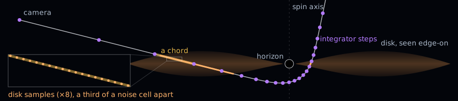
Charge enters only through $\eq{f}{f}$f‘s numerator, $2Mr - \eq{Q}{Q}^2 = 2r\,(M - \eq{Q}{Q}^2/2r)$2 M r minus Q squared equals 2 r times M minus Q squared over 2 r: at radius $r$r the geometry is that of a mass $M - \eq{Q}{Q}^2/2r$M minus Q squared over 2 r, since the energy $\eq{Q}{Q}^2/2r$Q squared over 2 r of the electric field outside $r$r is part of $M$M and pulls nothing inward. Charge therefore shrinks the outer horizon, the photon orbits and the shadow: without spin, as $\eq{Q}{Q}$Q approaches $M$M, the shadow’s radius falls from $3\sqrt{3}M \approx 5.2M$3 root 3 M, about 5.2 M to $4M$4 M. Photons carry no charge and the model’s gas is neutral, so the charge acts through the geometry alone. Holes in nature are close to neutral, since a charged hole draws opposite charge from the gas around it.

The horizons sit at

which exist only while $\eq{a}{a}^2 + \eq{Q}{Q}^2 \le M^2$a squared plus Q squared at most M squared. At the site’s spin the charge can reach only about $0.08M$0.08 M, too little to see, so the sliders lower the spin as the charge rises. Outside the outer horizon lies the ergosphere, where the spin drags spacetime around so strongly that nothing can stay still relative to the distant stars.

The shadow’s edge is light that grazes the unstable spherical photon orbits, whose radii run from the prograde to the retrograde orbit in the disk plane. An orbit of radius $r$r fixes, in closed form, two conserved quantities per unit energy: the photon’s angular momentum $\xi$xi about the spin axis, and its Carter constant $\eta$eta, which measures how far its motion carries it out of the disk plane. A distant camera at inclination $i$i from the spin axis sees that orbit’s light at the screen position $(\eq{X}{X}, \eq{Y}{Y})$X, Y, in units of $M$M from the hole’s center (the literature writes them $\alpha$alpha and $\beta$beta),

Prograde orbits lie closest to the hole, so the edge on the side turning toward the camera moves in and the shadow flattens there [7]. The shader never uses these formulas: its shadow is where its traced rays fall in. That makes them an independent test of the trace, and the CPU port of its integrator puts the shadow’s edge within a fraction of a pixel of theirs.

The disk’s light

Where a photon crosses the disk, the gas orbits at the Keplerian angular speed, which without charge is Bardeen, Press and Teukolsky’s [8],

and the ratio of observed to emitted frequency is

where $u^t$u upper t is the gas’s time dilation [9]. The factor $1/u^t$1 over u upper t holds the gravitational redshift and the transverse Doppler shift of the orbit, and $1 - \eq{Omega}{\Omega}\,\eq{xi}{\xi}$1 minus Omega xi the Doppler shift of the gas’s motion along the photon. The Schwarzschild formula above is this case without spin or charge.

Here the innermost stable circular orbit lies at $r_\text{in} \approx 1.28M$r in, about 1.28 M, close to the horizon. For other spins and charges it follows from a closed-form condition [10].

The disk is dim and starved, the kind a massive hole fed slowly has, and two heat sources set its temperature, $\eq{T}{T}^4 = \eq{Tv}{T_v}^4 + \eq{Tl}{T_l}^4$T to the fourth equals T v to the fourth plus T l to the fourth. Friction in the orbiting gas gives the thin-disk profile of the Schwarzschild model, $\eq{Tv}{T_v}$T v. Light from the inner disk falls on the outer disk where it flares, and this heating, $\eq{Tl}{T_l}$T l, falls off more slowly with radius:

with $\eq{Tl}{T_l}$T l switched on smoothly where the disk starts to flare.

Each sample glows as a black body at the observed temperature $\eq{g}{g} \eq{T}{T}$g T. The shader evaluates Planck’s law for photons of three energies $\eq{Ec}{E_c}$E c, the display’s red, green and blue, relative to a black body at the temperature $T_0$T zero of the display’s white:

where $k$k is Boltzmann’s constant. This contains the Schwarzschild model’s $\eq{g}{g}^3$g cubed: a black body’s specific intensity obeys $\eq{g}{g}^3 I_\nu(\nu/\eq{g}{g}, \eq{T}{T}) = I_\nu(\nu, \eq{g}{g}\eq{T}{T})$g cubed times I nu at frequency nu over g and temperature T equals I nu at frequency nu and temperature g T, so a black body shifted by $\eq{g}{g}$g looks exactly like one at $\eq{g}{g}\eq{T}{T}$g T. The result is linear radiance, and the frame’s bloom and tone curve act as the camera.

At these temperatures the display’s wavelengths lie on the steep, short side of Planck’s curve, where a change in temperature changes the brightness a lot and the color little. The Doppler shift therefore shows mostly as brightness. At $10M$10 M, gas moving straight toward an edge-on camera looks 150 times brighter in green than gas moving away. The side turning toward the camera glows gold-white and overexposes into the bloom, and the receding side dims to a deep orange that reads as brown. The film Interstellar left these Doppler effects out of its black hole’s disk, which with them would have looked as lopsided as this one [11].

The gas absorbs as well as it emits, more strongly in blue than in red, as dust does: its opacity grows with the photon energy. The accumulation sum $C \leftarrow C + (1 - A)\,a_i\,c_i$, from Tracing and marching, therefore runs once per color channel, and the near side of the disk hides and reddens what lies behind it.

The disk’s flow

The gas orbits at the Newtonian Kepler rate $\sqrt{M/r^3}$the square root of M over r cubed, close to $\Omega$Omega except near the inner edge, and drifts inward at a fixed fraction $\epsilon$epsilon of its orbital speed. Real gas falls in far too slowly to see, so I made it fall faster. Each parcel of gas therefore follows a trailing logarithmic spiral. To move the texture with the gas, the shader reads the noise at two quantities that stay the same for a parcel all along its path:

where $\varphi$phi is the angle around the spin axis in the direction the gas orbits, $t$t the time, and $t_\text{in}(r)$t in of r how long gas at radius $r$r takes to fall in. The first quantity says which spiral a parcel rides, and the second the moment it will reach the inner edge. Together with the height above the midplane they pick out one parcel, so each feature of the noise travels with its parcel, orbiting and falling in. Unlike a texture carried on circular orbits, it never winds up, so it needs none of the Schwarzschild disk’s restarting layers.

The gas is two octaves of that noise, $n$n. A smoothstep of $n$n gathers it into streaks along the spirals, with clear lanes between them. The streaks are densest at the midplane, and never denser than the captured matter allows. A third, coarser octave makes the top of the gas billow. The gas fills a lens-shaped slab, thin at the inner edge and at the rim and thickest about halfway out. Its temperature follows the noise too, so the dense streaks run hotter.

Three hot spots orbit near the inner edge, compact flares like those the GRAVITY instrument tracked around Sagittarius A* [12]. Each lives a few orbits and heats the gas to up to twice the disk’s temperature, so it flashes as it swings toward the camera, and its lensed image sweeps around the shadow.

A thin corona, hot plasma that scatters the inner disk’s light, glows in a ring just outside the photon orbits. It emits light without absorbing any. The shader samples it along every chord, so it is lensed like the disk: its near side crosses the shadow as a thin band, and its light bent around the hole rims the shadow’s edge.

Tracing Kerr–Newman in real time

This part is engineering rather than physics: the shortcuts that let the trace keep up with the frame rate. Integrating every ray through the full metric is the heaviest work on the site.

The traced image’s size follows the computer’s speed. Every few frames the trace compares the median frame time with a target, and it traces more pixels when frames run well ahead of it and fewer when they fall well behind. The target drops once the close-up has settled: a slow computer gives up frame rate for a sharper settled disk, which changes little from frame to frame.

Each frame jitters the rays by a fraction of a pixel and blends the new image $C_\text{new}$C new with the previous result $C_{t-1}$C t minus 1, the history [13],

an exponential average with a time constant of ten frames. Each frame’s rays land at slightly different points in their pixels, so the average covers each pixel’s whole area and smooths its edges. Between frames the view only moves and scales about the hole, which lets a pixel at screen position $\eq{q}{\vec{q}}$vector q find its previous value at

where $\eq{c}{\vec{c}}$vector c is the hole’s screen position, $\eq{s}{s}$s the view scale, and primes mark the previous frame. This follows the view, not the gas, so moving gas would leave a trail of its earlier positions, called ghosting. The standard guard clamps the history to the range of colors around each pixel in the current frame [13].

Near the shadow, lensing squeezes a large stretch of disk into a few pixels, and a single ray per pixel turns that gas into grain. With $\eq{o}{\vec{o}}$vector o the offset from a pixel to the point of the sky its ray reads, the trace refines a pixel, adding rays to it, wherever

that is, wherever the offset changes by more than half a pixel from one pixel to the next. The test runs only where the previous frame showed disk or shadow nearby, since extra rays refine nothing else, and pixels along the shadow’s edge are always refined. A refined pixel traces its center ray and one of four sub-pixel rays, a different one each frame, and the history blend averages them along with the jitter.

Refinement is where the trace spends instead of saves: it takes about a quarter of the trace’s time. Tracing all four sub-pixel rays every frame on the photon ring (the thin bright ring that hugs the shadow) and at the shadow’s edge, at full resolution, can make a single frame on a laptop take long enough for the browser to reset the GPU, and after a few resets it turns WebGL off.

Most of a ray’s path runs through empty space. Before each sample the shader computes a safe distance to the nearest gas, whether the ray is above the slab, beyond its rim or in the gap inside the innermost stable orbit, and jumps that far at once. No other shortcut saves as much: without it the trace takes twice as long.

A ray that meets the dense midplane stops early, since the gas there turns opaque within a few samples. Without that stop the trace takes about a fifth longer. A ray crossing the thin gas above and below the midplane samples all the way through, and those rays are the expensive ones.

Along each chord the shader spaces the gas samples by how fast the ray crosses the gas’s structure, across the streaks and up through the billows: a fraction of a noise cell apart, and at most a fixed number on each chord. Where that limit leaves them sparser, on chords that graze the disk, the octaves finer than their spacing fade out, as in the Schwarzschild disk, and the gas blurs instead of aliasing into false patterns. Each frame’s jitter shifts where the samples land, and the history blends about ten frames of them.

The noise is cheaper than it looks. Each octave blends random values at the eight corners of a lattice cell. Instead of computing them with a hash, the shader stores the lattice in a small texture, two neighboring slices in its red and green channels. The texture hardware blends neighboring entries for free, so one read returns the blend of a cell’s four corners in both slices. The lattice repeats, with a period the disk’s spirals hide. With an ordinary sine hash at the eight corners instead, the trace takes over a third longer.

The last shortcut acts only while the hole’s image is small. A ray passing farther than $48M$48 M from the hole cannot reach the disk, so instead of being integrated it takes the weak-field bend of an uncharged hole without spin, to second order [14],

where $\eq{b}{b}$b is the ray’s impact parameter and $\eq{psi}{\psi}$psi the angle at the camera between the ray and the direction to the hole. For a distant camera $\eq{psi}{\psi}$psi is small at a given $\eq{b}{b}$b, and the first term tends to $4M/\eq{b}{b} = 2R_s/\eq{b}{b}$4 M over b, which is 2 R s over b, the bend derived for the Schwarzschild model. The camera is not infinitely far away, so part of the pull lies behind it. The factor $1 + \cos\eq{psi}{\psi}$1 plus cosine psi keeps only the part ahead of it: exactly for the first term, approximately for the second. Spin and charge add terms of the same order to the full bend, $\mp 4\eq{a}{a}M/\eq{b}{b}^2$minus or plus 4 a M over b squared for a ray in the disk plane [15] and $-3\pi\eq{Q}{Q}^2/4\eq{b}{b}^2$minus 3 pi Q squared over 4 b squared [14], which the shader leaves out. At $48M$48 M both are small. In the held close-up the $48M$48 M circle lies beyond the screen’s corners, and by the time it comes on screen the error is about two pixels and shrinks with the image.

What is physical and what is design

In both black holes, light follows general relativity, to the accuracy measured above. The Schwarzschild model reads the exact orbit equation’s paths from its table, and its disk’s redshift is exact for circular orbits. Its camera takes each pixel’s direction as a straight line, so it shows the image slightly larger than a camera at rest that close to the hole would see it. The Kerr–Newman camera measures directions as one at rest does. The Kerr–Newman model integrates the geodesic equations for any spin and charge a hole can have, its disk fades in across the exact innermost stable orbit, and its gas glows as a black body at the redshifted temperature, sampled at three wavelengths where a camera would weigh the whole spectrum through its color filters. It leaves part of the work to a weak-field bend, which it uses alone for rays that pass farther than $48M$48 M from the hole. The matter grid conserves mass exactly, however long the disk turns.

Everything else invokes artistic freedom: the starfield and its diagrams, the galaxy, its intro and its helix, the meteors and comets with their trails, the capture, the gas textures, the Schwarzschild disk’s palette and brightness, the Kerr–Newman disk’s temperatures, its quick inflow, its hot spots and its corona. Several of these borrow a physical law as a model, such as the pinhole camera’s depth scaling, a diffusing puff’s width or Kepler’s third law, and depart from it where the picture calls for it.

Where the blog went

The plan was a blog with a few stars behind it. The stars are now about half of the site’s code, nine tenths with the demos that explain them, and this post is entirely about them. The next one will be about something else.

References

1. Inigo Quilez, Domain warping.
2. Frederic H. Vincent, Thibaut Paumard, Eric Gourgoulhon and Guy Perrin, GYOTO: a new general relativistic ray-tracing code, Classical and Quantum Gravity 28, 225011 (2011).
3. Riccardo Antonelli, Starless: a black hole raytracer.
4. Jean-Pierre Luminet, Image of a spherical black hole with thin accretion disk, Astronomy & Astrophysics 75, 228 (1979).
5. Nikolai I. Shakura and Rashid A. Sunyaev, Black holes in binary systems: observational appearance, Astronomy & Astrophysics 24, 337 (1973).
6. G. C. Debney, R. P. Kerr and A. Schild, Solutions of the Einstein and Einstein–Maxwell equations, Journal of Mathematical Physics 10, 1842 (1969).
7. Volker Perlick and Oleg Yu. Tsupko, Calculating black hole shadows: review of analytical studies, Physics Reports 947, 1 (2022).
8. James M. Bardeen, William H. Press and Saul A. Teukolsky, Rotating black holes: locally nonrotating frames, energy extraction, and scalar synchrotron radiation, The Astrophysical Journal 178, 347 (1972).
9. C. T. Cunningham, The effects of redshifts and focusing on the spectrum of an accretion disk around a Kerr black hole, The Astrophysical Journal 202, 788 (1975).
10. Daniela Pugliese, Hernando Quevedo and Remo Ruffini, Equatorial circular orbits of neutral test particles in the Kerr–Newman spacetime, Physical Review D 88, 024042 (2013).
11. Oliver James, Eugénie von Tunzelmann, Paul Franklin and Kip S. Thorne, Gravitational lensing by spinning black holes in astrophysics, and in the movie Interstellar, Classical and Quantum Gravity 32, 065001 (2015).
12. GRAVITY Collaboration, Detection of orbital motions near the last stable circular orbit of the massive black hole SgrA*, Astronomy & Astrophysics 618, L10 (2018).
13. Lei Yang, Shiqiu Liu and Marco Salvi, A survey of temporal antialiasing techniques, Computer Graphics Forum 39, 607 (2020).
14. Charles R. Keeton and A. O. Petters, Formalism for testing theories of gravity using lensing by compact objects: static, spherically symmetric case, Physical Review D 72, 104006 (2005).
15. Mauro Sereno and Fabiana De Luca, Analytical Kerr black hole lensing in the weak deflection limit, Physical Review D 74, 123009 (2006).